f2py gcc.exe: error: CreateProcess: No such file or directory

Again, for unclear reasons my f2py stopped working. Scripts that I could compile previously could not be compiled anymore. Without knowing why it stopped working, or why my proposed fix worked, I just wanted to let you know that I did to get f2py to work again on my windows x64 pc for python 2.7.

• Upgrade to the latest Python version (for me 2.7.10 worked). Download and install:
• https://www.python.org/downloads/release/python-2710/
• Remove the old mingw version and download and install:
• http://sourceforge.net/projects/mingw-w64/
• (make sure when you install, the arcitecture flag is set to "x86_64")
• Open the system environment variables, remove old references to mingw, and add the '.../mingw/bin' path to your Path variable. For me that was "C:\Program Files\mingw-w64\x86_64-5.3.0-posix-seh-rt_v4-rev0\mingw64\bin"

Optionally restart the pc or open a new DOS shell and run f2py. This worked for me.

wxOpenGL frame work for rendering numpy data

wxOpenGL framework

This frame work lets you render and dynamically modify numpy data (quad-, triangle-meshes) via provided wxOpenGL framework. 

Application functions (keyboard keys):
+ E - Toggle edge visibility

Application functions (viewport manipulation):
+ Middle mouse button & mouse motion - rotate opject
+ Mouse wheel - Zoom
+ Ctrl & Middle mouse button & mouse motion - rotate object
+ Shift & Middle mouse button & mouse motion - translate object

The framework can be downloaded at:
https://www.dropbox.com/sh/ip306uavm7jpekg/2adXHWODU1

The package contains the application (wx_opengl.py) and a render object class (render_object.py) which may be used to add triangle / quad data and meshed to the application viewport. 

Affine Image Registration (follow up, a feature-based approach)

This is a follow up on the previous rigid image registration approach. In the following example I am showing you how to implement an affine transformation registration based on image features with python. In our lab we quite often have to analyze pharmacokinetic parameters based on transient fluorescence imaging taken from tissue in an animal skin flap window. It is the nature of tissues to move during the imaging recording process especially when heat is applied to the tissues. To correct the movement between the individual images, a affine transformation approach is presented to correct the images. 

In a first step, the gradient images are derived from the original images and "landmark" features are detected via threshold criteria (Figure 1).

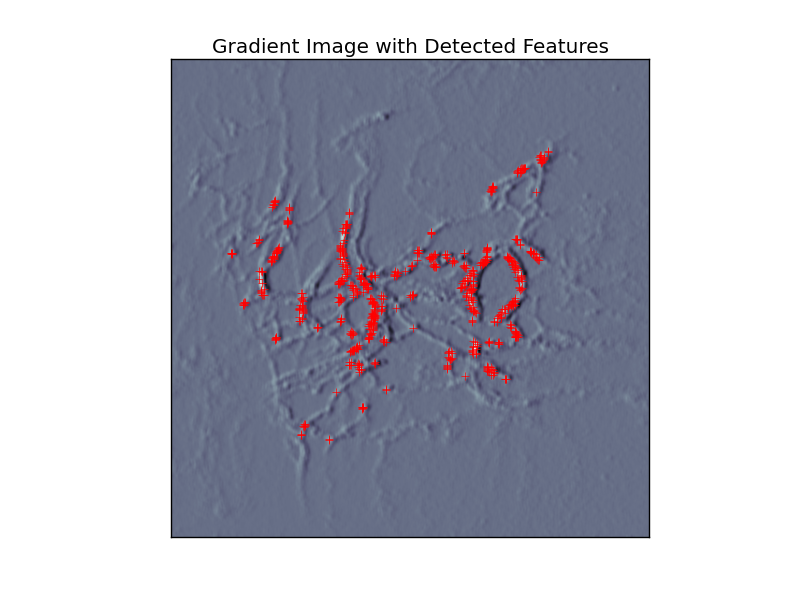
Figure 1

In a second step, affine transformation is applied to the matching image via optimization method until a defined distance criteria (nearest neighbor criteria with KDTree) between the landmarks reached a minimum (Figure 2).

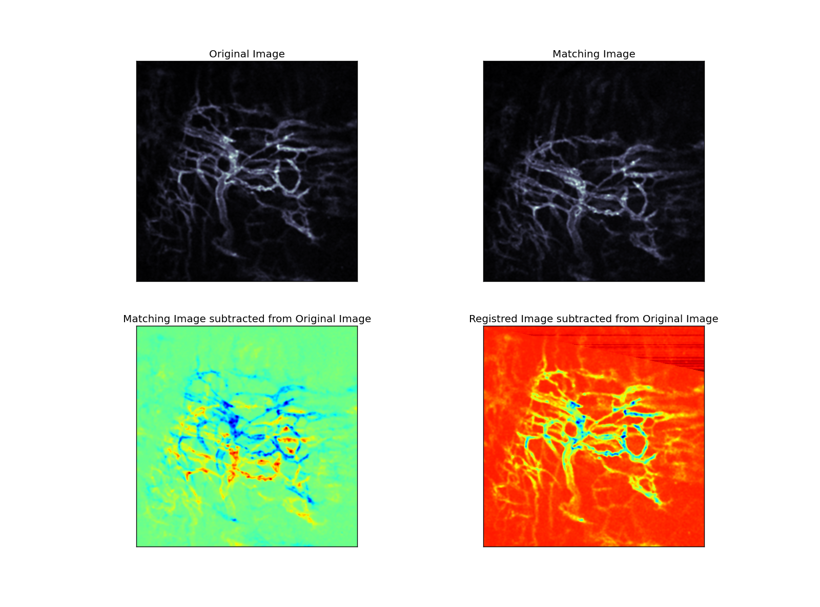
Figure 2

The Python code:

       
'''
@author: Christian Rossmann, PhD
@license:  Public Domain
@blog: http://scientificcomputingco.blogspot.com/
'''

from scipy import ndimage
from scipy.spatial import cKDTree
from scipy.optimize import fmin

def register(im1,im2):
    
    # initialize the transformation matrix
    T = [[1.0,0.0],[0.0,1.0]]
    
    # extract features from first image  
    edges1 = ndimage.sobel(im1)
    features1 = dstack(where(edges1.T > edges1.mean()))[0]
    kd = cKDTree(features1)
    
    def errfunction(T,kd=kd,im2=im2):
        
        # transform the image
        img = ndimage.interpolation.affine_transform(im2,T.reshape(2,2))
        
        # extract features from transformed image 
        edges = ndimage.sobel(img)
        features = dstack(where(edges.T > edges.mean()))[0]
        
        dst,idx = kd.query([features])
        
        # measure the distances between features.
        return sum(dst**2)
        
    T = fmin(errfunction,T,xtol=1.e-6,ftol=1.e-6,maxfun=5000,maxiter=5000)
    
    return (T,ndimage.interpolation.affine_transform(im2,T.reshape(2,2)))

im1 = imread("sample_images/IMG1.png")[:,:,0]
im2 = imread("sample_images/IMG2.png")[:,:,0]

im1 = ndimage.filters.uniform_filter(im1,5)
im2 = ndimage.filters.uniform_filter(im2,5)

im1 -= im1.min(); im1 /= im1.max() 
im2 -= im2.min(); im2 /= im2.max()

(T,rimg) = register(im1,im2)

#%%
figure(1)
clf()
s = subplot(1,1,1)
title('Gradient Image with Detected Features')
imshow(edges,'bone')
edges = ndimage.sobel(im1)
features = dstack(where( (edges.T > 0.45) & (edges.T < 0.55) ))[0]
plot(features[:,0],features[:,1],'+',color='red')
xlim([0,im1.shape[0]])
ylim([0,im1.shape[1]])
s.axes.get_xaxis().set_visible(False)
s.axes.get_yaxis().set_visible(False)
#%%
figure(2)
clf()

s = subplot(2,2,1)
title('Original Image')
imshow(im1,'bone')
s.axes.get_xaxis().set_visible(False)
s.axes.get_yaxis().set_visible(False)

s = subplot(2,2,2)
title('Matching Image')
imshow(im2,'bone')
s.axes.get_xaxis().set_visible(False)
s.axes.get_yaxis().set_visible(False)

s = subplot(2,2,3)
title('Matching Image subtracted from Original Image')
imshow(im2-im1,'jet')
s.axes.get_xaxis().set_visible(False)
s.axes.get_yaxis().set_visible(False)

s = subplot(2,2,4)
title('Registred Image subtracted from Original Image')
imshow(rimg-im1,'jet')
s.axes.get_xaxis().set_visible(False)
s.axes.get_yaxis().set_visible(False)

show()

Rigid Image Registration (a quick & dirty intensity-based approach)

Fig. 1. Showing the original image, the manual transformed, and the automatically corrected image via registration algorithm.

Image registration is useful when you want to compare different images from the same object but taken from different angles. In order to make the images comparable, one has to correct the transformation of the target images, so that the target images align with the reference image. This is a quite useful technique with a broad range of applications. One of them is in Medical Imaging where images of the same anatomical structures are taken with different modalities and at different time points.
In this example I am loading good old Lena into the application to demonstrate the function of the code. The important part of this implementation it the finding of initial values (guess) for the fmin (optimization-) function. Without that step, the function is very likely not able to find the correct transformation parameters. Thus, to provide an initial guess, I let the x,y (image shift) and the r (image rotation) vary from -10 to 10 and calculate the intensity-based image errors. Subsequently, the minima for these variations are determined and used as initial guess. (Maybe not the best method but quite simple and robust). Then, I pretty much let the fmin function do the magic to search for the parameters that yield the smallest value returned form the intensity-based image error function.    

The Python code:

       
'''
@author: Christian Rossmann, PhD
@license:  Public Domain
@blog: http://scientificcomputingco.blogspot.com/
'''

import numpy as np
import Image
from scipy import ndimage
from scipy import optimize
from scipy import misc

from pylab import *

def MeasureErr(img1,img2):
    diff = (img1-img2)
    return sum(diff**2)

def RigidRegistration(img,ximg):
    
    # Perform initial guess rotation & translation 
    v_range =  np.array(xrange(-10,10))
    
    err = np.array([MeasureErr(img,ndimage.shift(ximg,(v,0))) for v in v_range])
    x = v_range[where(err==err.min())[0]]
    
    err = np.array([MeasureErr(img,ndimage.shift(ximg,(0,v))) for v in v_range])
    y = v_range[where(err==err.min())[0]]

    err = np.array([MeasureErr(img,ndimage.rotate(ximg,v,reshape=0)) for v in v_range])
    r = v_range[where(err==err.min())[0]]

    # List contains displacement in x and y and rotation
    
    param = [x,y,r]
    
    def ErrFunc(param,img=img,ximg=ximg):
        
        # Perform rotational and translational transformation
        
        _img = ximg.copy()
        _img = ndimage.rotate(_img,param[2],reshape=0)
        _img = ndimage.shift(_img,param[:2])
        
        return MeasureErr(img,_img)

    
    param = optimize.fmin(ErrFunc,param)
    
    #Final transformation
    _img = ximg.copy()
    _img = ndimage.rotate(_img,param[2],reshape=0)
    _img = ndimage.shift(_img,param[:2])
    
    return (_img,param)

img = misc.lena().astype('float32')

# Normalize image (0-1)
img -= img.min() 
img /= img.max()

# Generate transformed image
ximg = img.copy()
ximg = ndimage.shift(ximg,(5,-1))
ximg = ndimage.rotate(ximg,-4,reshape=0)

(rimg,param) =  RigidRegistration(img,ximg)

 
figure(1)
clf()
subplot(1,3,1)
title('Original')
imshow(img)
subplot(1,3,2)
title('Transformed')
imshow(ximg)
subplot(1,3,3)
title('Registered')
imshow(rimg)
show()

Optimizing radiofrequency ablation heating strategies for localized drug delivery from thermosensitive liposomal doxorubicin

This is my poster for the MUSC HCC Retreat 2013.

Python Spyder, clear workspace/shell command

Python Spyder is a great Tool similar to Matlab but still lacking commands for clearing variables form workspace. I've added following code to the Spyder startup file (C:/Python27/Lib/site-packages/spyderlib/scientific_startup.py) to generate clear commands for workspace and the shell:

So whenever I type clear() or clear_all(), the command shell or the variables from the workspace will be cleared, respectively.

Cancer treatment with Doxorubicin (a mathematical model)

Cytotoxic antineoplastic drugs are administered to treat many different types of cancer including breast, lung, bladder and liver cancer. Doxorubicin (DOX) is a chemotherapy agent (also called Adriamycin) which is given by injection or drip (infusion) through a fine tube inserted into the vein (e.g. cannula), through a fine plastic tube inserted into a vein near your collarbone (central line) or into a vein in the crook of your arm (PICC line). Mathematical modeling can be used to determine DOX drug concentration in in systemic plasma, aggregate body tissue, tumor plasma, tumor interstitial space, and tumor cells. Such mathematical models allow optimization of drug delivery systems to achieve a better therapeutic index.

In the section below I present a mathematical model according to (http://www.musc.edu/ablation/pubs/Gasselhuber,%20PLos%20One%202012.pdf) to predict systemic and tumor drug concentrations for DOX in mice.

Overview about the mathematical model including compartments for body plasma, body tissue, tumor plasma, extra and intracellular compartment for tumor tissue. The transport mechanism between the compartments are indicated via arrows.

The ordinary differential equation model was built and solved via Python.